Car localization by CNNs

Computer Vision has improved a lot ever since the emerge of Deep Learning. One thing that always struck me as odd however, is how many tutorials cover image classification only, while in reality you would almost always need not just classification but localization as well. So I was really excited when I finally tried object detection and localization myself when the vehicle detection and tracking project of the Udacity self driving car nanodegree (together with nicely assembled training data) came along. While Udacity’s lessons focus on classic computer vision techniques like extracting HOG features, there is no reason to stop there and not try to use the same data to train a convolutional neural network (CNN). This is what this post will be about. I will assume that you are already familiar with CNNs for classification — otherwise check one of the many tutorials on that.

There is one feature of CNNs that make using them for localization very interesting: CNNs can be very fast as they allow you to reuse a lot of intermediate data. This way a relatively dense sliding window approach actually becomes feasible even on lower end hardware. Foundations

In principle it is possible to view localization just as a a matter of running the classifier on all possible locations of the image and generating probabilities for each of them. Needless to say that means that the classifier has to run may times per image which is slow. That is why in traditional CV you would usually want to have some guesses where you will probably get detections and not run the classifier everywhere. So why does it work for CNNs? Fig. 1 shows a representative CNN classifier, the important thing to realize here is that the convolutional layers are not limited to any specific size you can run convolutional filter on arbitrarily large images and all that changes is that you get larger feature maps out. The only place where we really need to know the size in advance are the final dense layers. So how can we solve that? Turns out the easiest way to do it is to replace them with convolutional layers as well. Why is that possible? Think of if this way: If you have an dense layer running on a (flattened) 64x64 image and generating 10 output nodes that really is no different from a convolutional layer with height and width of 64 and output dimension of 10. The only difference it that this layer will also run on 65x65 just producing 4 output values. The beauty of this approach is that you can basically take any CNN classifier, turn it in to a localizer and reuse all the generated by the upper layers.

Softmax

There is one more thing to consider: what about Softmax? If you remember the equation to calculate softmax

you notice the normalization term. When you use this with CNN output you clearly do not want to normalize over all output points at the same time as this would be incorrect. Your final layer gives you something like output[batchsize,x,y,numberof_classes] as compared to the usual output[batchsize,numberof_classes]. To my knowledge at least in keras there is no ready made function/layer for it but it is easy enough to implement a custom softmax: instead of calculating the result of equation 1 once, you have to do it for each point x and y and normalize along the last axis. That can be easily implemented as a custom layer in keras — and actually other people have done it before and it can be found on github (it also explains on how to use pre-trained weights with this method, but for our problem of just detecting car/not car a full alexnet trained on imagenet is inefficient). On the other hand first thing you should ask yourself is: do i really need softmax? If you have a binary problem like in our case is the sample a car or not the answer is no, you can simply use a tanh output layer with -1 being class 1 and +1 being class 2.

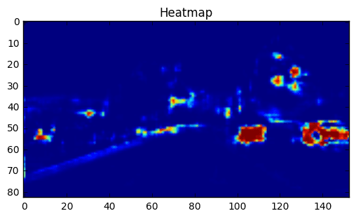
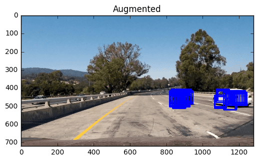
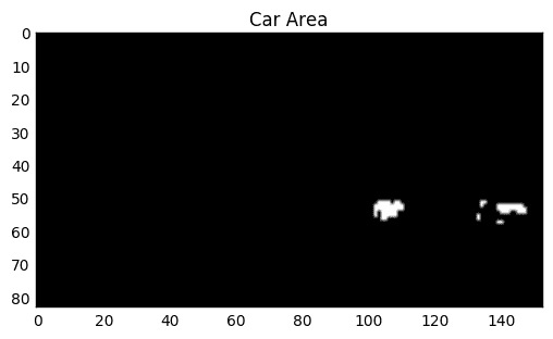
At this point let’s have a look at a practical implementation of the car not car network (check out the github repository). As usual I load the samples first, separate a small validation set (small because its not the metric we are really after anyway). The model is also simple just 2 3x3 convolutional layers with relu activation followed by 8x8 max pooling, a 8x8 convolutional layer to replace a dense layer with 128 output nodes, and a final dense layer converting it all to just one output value (although in 4d) if a 64x64 input image is used. Now to actually train this, I need a fixed output size and since the training samples provided by Udacity are 64x64, the input shape is 64x64x3 for training. This also allows me to add a flatten-layer and then use keras’ usual fit function. After training, I save the weights and create a new network with the shape None x None x 3, no flatten layer in the end and the same weights. That is it. And in my opinion that is the whole beauty of this approach: you don’t need crazy hardware to train it and you can easily adapt classification networks. It also runs really fast with more than 30fps. For demonstration let’s run the network on a sample image (Fig. 2). The output is a heat map (Fig. 3)— now we can clearly see that not everything that shows up in there is really a car, the low confidence areas are often not but it is pretty confident about the car so lets use that to our advantage and use a quite high threshold of 0.99.

With that we only get the car area. One thing to also keep in mind is that we do 8x8 max pooling in the model after the 2 convolutional layers. This is important if we want to figure out what patch in the original image a pixel in the heat map corresponds to. If we have the coordinates i,j in the heat map they correspond to the rectangle [(i8,j8), (i8+64,j8+64)] in the original image. We can use this knowledge to draw rectangles around the detected areas as shown in Fig. 5. Here, just like in many other detection methods we will need to merge duplicates into one, which is actually also a challenging problem but not the topic of this article. The most simple way to get rid of duplicate detections would be to use OpenCV’s groupRectangle but more sophisticated methods might work.

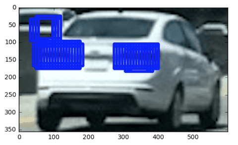
Now there is one last open question: what about very big cars can they be detected? If it is too big (to much in the foreground, Fig. 6) it does not work well. In this case the only solution is to run the same classifier on a resized image but as long as it is within reasonable boundaries (Fig. 7) it actually performs quite well anyway.

To conclude I have shown how to use CNNs to efficiently generate heat maps to localize cars in images using a simple method that can be derived easily from classification methods.

Update: In my view this is also one of its major advantages over more sophisticated methods, such as YOLO, SSD or RCNN. You can train it with a very limited dataset and it is very computationally efficient you should just not expect it to be able to do the same things. It is surprising how well it worked for me for many tasks besides this one.

This is a repost from something I originally posted at medium