AI based CBC

This article will give some background using deep reinforcement learning for coherent beam combining. I recently published an Optics Express Article on this topic which covers the potential for CBC. As it is open access there is no point in writing the same again here. The article is about the potential of reinforcement learning in the context of optics and CBC since reinforcement learning by itself is not new. However, optical scientists might still be interested in the fundamentals of reinforcement learning so this is what this article will be about.

A very brief summary

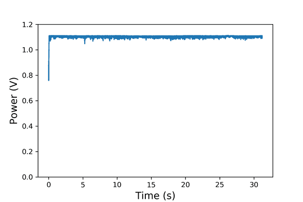
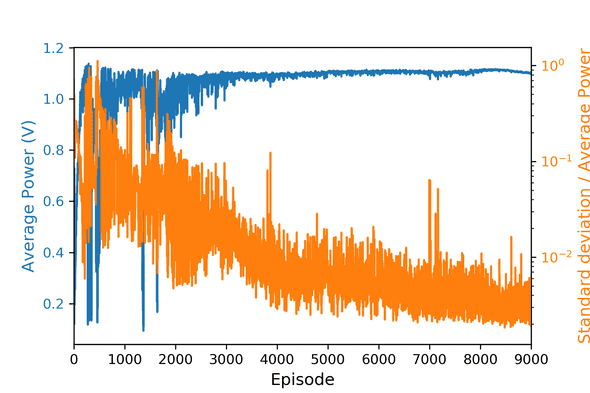
The idea behind reinforcement learning for CBC is very simple: instead of designing your controller you use a general purpose method - reinforcement learning - which will try out random actions based on an observed state and iteratively optimize a reward function. Once this is done one can then hopefully use this learned program maximize the reward function based on the state and in fact do CBC. We have shown that this is possible by combining two lasers experimentally as seen in Figure 1 and 2.

How to do it?

As many optical scientists most likely are not as familiar with computer science / artificial intelligence I will try to capture the this as a supplement to the article - or conference talks I have given - here.

Reinforcement learning tries to learn the optimal action $a_t$ (in case of CBC this is the actuator movement) given a state $s_t$ at time $t$, in order to maximize a total future reward $r$. The state $s_t$ is either directly an observation or modified by an observation. Each such pair of actions and states one can then be assigned a value $Q(s_t,a_t)$. The better the action $a_t$ in state $s_t$ the higher the $Q$. This means if we know $Q$ we can determine the best possible action action $a_{t,opt}$ because $Q(s_t,a_{t,opt}) = \max\limits_{a_t} Q(s_t, a_t)$. The problem is we do not know $Q$ of course. We can approximate $Q$ by starting with a random $Q$ and iteratively making it better by applying

Here, $\alpha$ is the learning rate - which determines how fast we change $Q$ at each step and $\gamma$ is the discount factor which, all other things being equal, accounts for the fact that we care more about rewards now than in the future. It has to be less than 1 for stability. We can represent $Q$ as a neural network in this case we can simply turn the problem to the usual supervised learning form with observations x and targets y. Those are easy to calculate if we have $s_t,s_{t+1},r_t$ and the neural network $Q$ calculates a vector of values representing the potential actions:

In practice there are two potential problems here: Neural networks assume uncorrelated samples when training. This will never be true for reinforcement learning as samples collected at similar times will always be highly correlated. To avoid this we need to save the $s_t,s_{t+1},r_t$ values and sample form the old data pool to get uncorrelated observations. There are more advanced methods which prefer to use samples with high error but simply taking random state action pairs from the buffer is enough.

The second potential problem is that we use $Q$ to calculate $y$ which we then use to update $Q$, which can become unstable. To stabilize this is can be a good idea to use two $Q$ networks.

Congratulations at this point we have deep reinforcement learning as used in Atari or Alpha Zero, although it is just a small part of these systems.

But we need analog output!

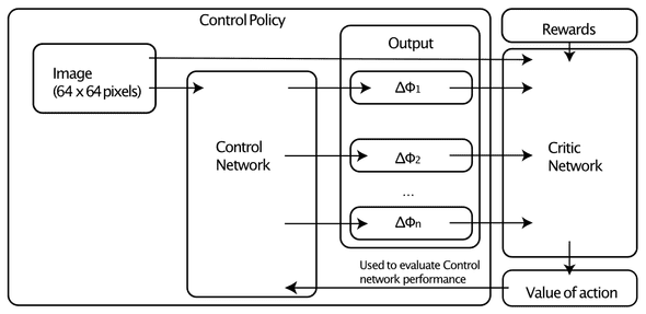
Indeed. The most simple way to get this is by discretizing and mapping the analog values onto a vector of finite numbers. This was the first method we used in. While this works, there are now much better - and more complicated architectures. Most notably the deep deterministic policy gradient. The general architecture of this scheme is shown in Fig. 3. Most notably we use two neural networks and the first neural network directly calculates the required analog action(s) with no maximization needed anymore. However as the above scheme for training then does not work anymore we need an additional neural network for training: the critic network. The critic network determines the $Q(s_t,a_t)$ as we know it where $a_t$ are now the actions given by the control network. And since the whole combination is differentiable we can then also use the optimizer to iteratively adapt the weights of the control network to maximize $Q$ (which is the same as optimization done by any neural network framework, only with a minus sign) while keeping the weights of the critic network fixed. So while this looks complicated (and is complicated in the details due to convergence etc…) the principle is not very difficult to understand.

Why is this better? First of all it gives the neural network more fine grained control over the output. But furthermore since the output now has less dimensions it usually also converges faster and to more reliable policies. There can still be challenges with convergence depending on the problem but for CBC this method works rather well. There are alternative methods as well for example proximal policy evaluation or more advanced DDPGs but this goes beyond this simple introduction.